Visual notes - intro to igraph

Balls and sticks

I think of network graphs as a bunch of balls and sticks, not unlike the magnetic building sticks my baby cousin plays with.

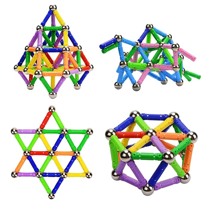
Ignore the top right example and you’ll find stellar examples of network graphs. The graphs can come in different shapes and sizes, and even in a rainbow of colors.

In real networks, the silver balls above may also come in varied sizes or colors or shapes. Sometimes the sticks become arrows, or be fat or thin. Using the official terminology, these “balls” are called vertices or nodes, and the “sticks” are called edges. The vertices, edges, or graph as a whole may have additional characteristics, or attributes, that describe them, such as size or group. A graph containing edges of different thicknesses, for example, is a weighted graph.

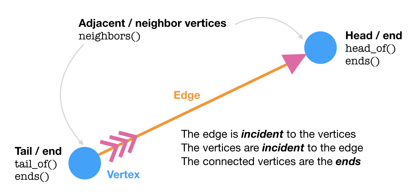
If we zoom in on a pair of vertices, we discover a bit more terminology. Edges are defined by the two vertices on each end of the edge. In a directed edge (with an arrow / has a direction), the vertex at the “arrowhead” is the head and the “feathered” vertex is the tail.

The igraph class

All the information about a network (e.g. those magnetic structures above) can be stored in an igraph object. A graph (g) in the network context is the combination of vertices and edges that make up a network. This does not refer to an actual plot, although you can also easily plot() a graph. (Confusing, I know.)

Seeing the output of the igraph object for the first time is a bit overwhelming, but this is what it is telling you:

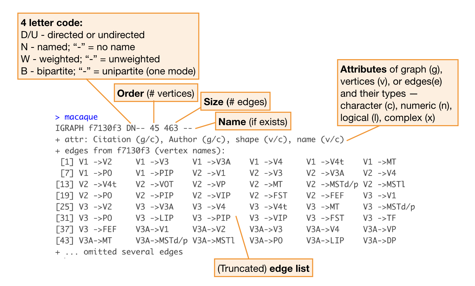
Note: The book makes extensive use of the igraphdata package, which includes several example igraph objects, such as the dataset macaque, shown above. This makes it easy to explore igraph class objects without creating one yourself.

Vertices and edges

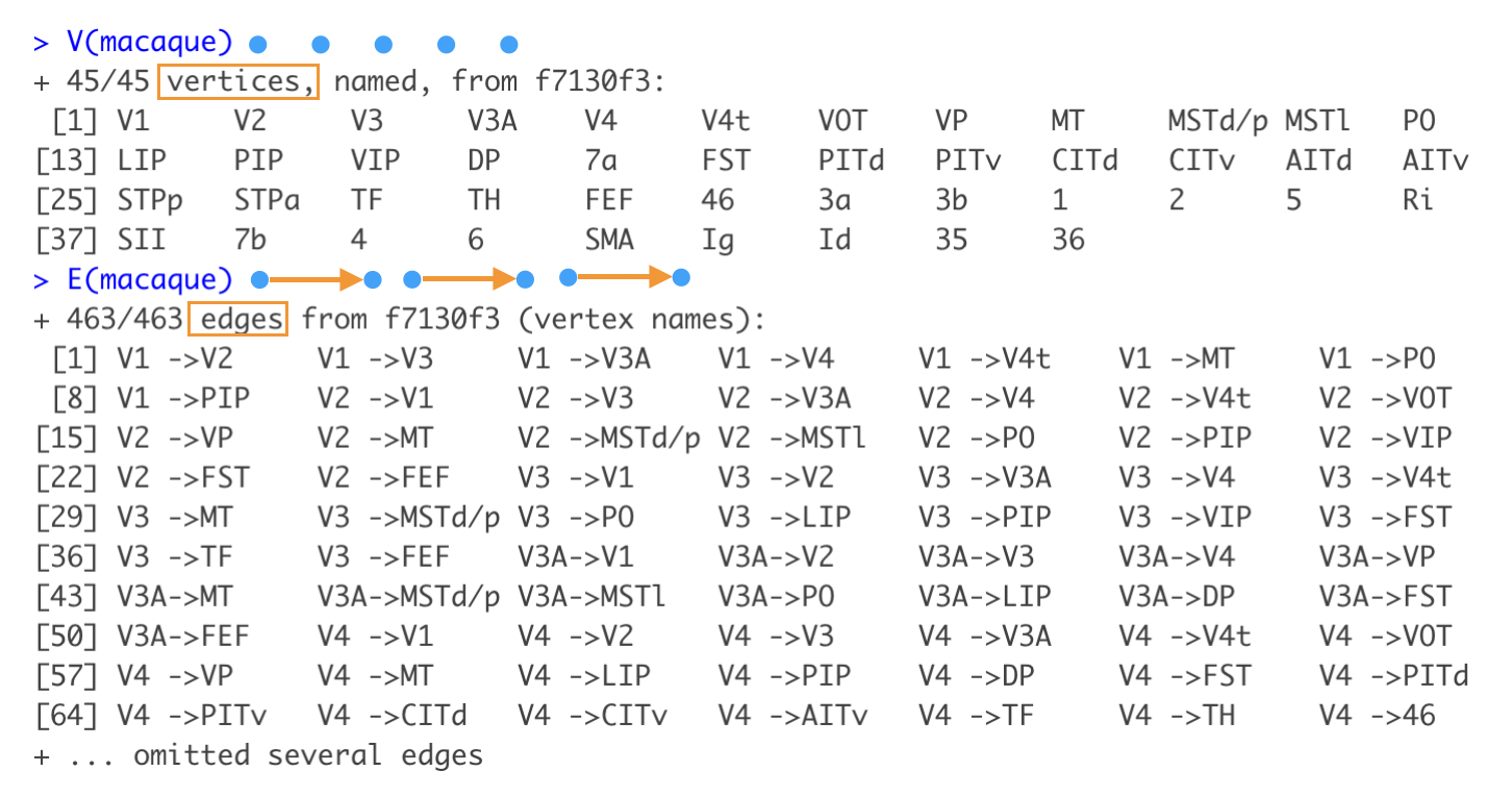
Once you have a graph object chances are, you’ll want to look at its parts and maybe modify it. The two basic parts of a graph are the vertices and edges, which you can extract with V() and E().

You can specify specific vertices/edges using their position or name:

V(macaque)[1]
V(macaque)["V1"]

E(macaque)[1]
E(macaque)["V1|V2"]

To remove or add vertices/edges to a graph, you can use your basic arithmetic operators. Subtracting is easy – just describe explicitly which vertices or edges you want to remove.

macaque - V(macaque)[1:42]

## IGRAPH 5db20f6 DN-- 3 4 -- 
## + attr: Citation (g/c), Author (g/c), shape (v/c), name (v/c)
## + edges from 5db20f6 (vertex names):
## [1] Id->35 Id->36 35->Id 36->Id

To add, you may need the vertices() or edges() functions. Note that edges can only connect existing vertices.

macaque - V(macaque)[1:42] + edges("Id","Id", "Id","35") 

## IGRAPH 968a671 DN-- 3 6 -- 
## + attr: Citation (g/c), Author (g/c), shape (v/c), name (v/c)
## + edges from 968a671 (vertex names):
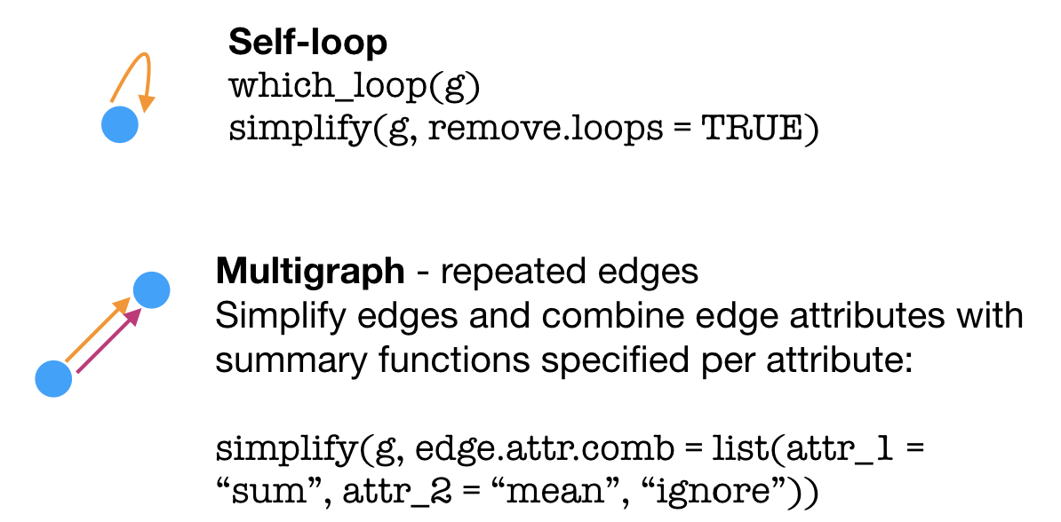
## [1] Id->35 Id->36 35->Id 36->Id Id->Id Id->35

macaque - V(macaque)[1:42] + edges("Id","a vertex that doesn't exist yet") 

## Error in as.igraph.vs(e1, toadd): Invalid vertex names

Like in the examples above, a graph may contain edges that are self-loops – a vertex connected to itself – or multigraphs (a.k.a. duplicated edges). You may sometimes need to simplify() a graph to use certain clustering functions (such as cluster_fast_greedy()) or do other analyses. This can mean removing loops, removing duplicate edges, or combining the attributes of duplicate edges using a summary functions.

Graph bits & pieces

Imagine standing on a vertex and starting to walk down an edge, continuing onto connected vertices and edges. The edges that you walk on make up what is called–surprise, surprise–a path. Often, network problems involve finding the shortest path(s), or geodesic, between two points (think flight connections, for example).

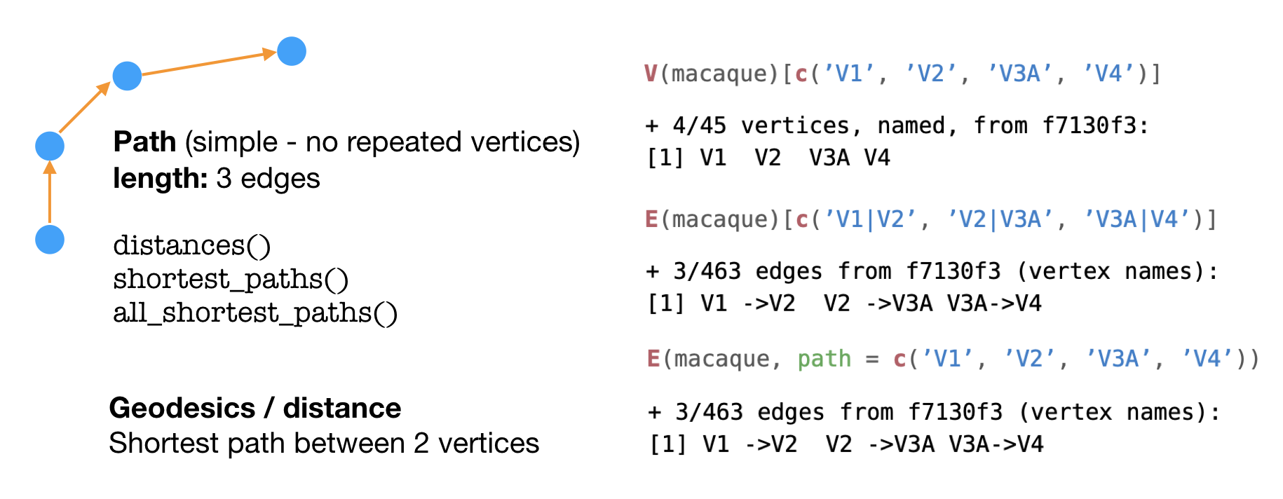
To extract a path from an igraph object, you can specify either the the vertices or edges that make up the path, as seen on the right above.

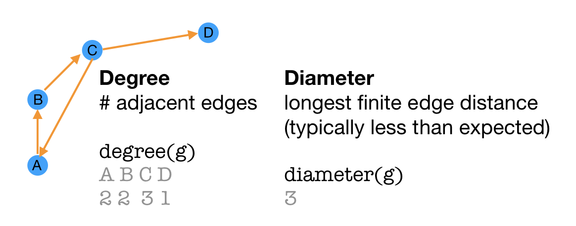
Degree is an attribute of a vertex that describes the number of adjacent edges. The shortest loop that can be made with the edges is the diameter of the graph.

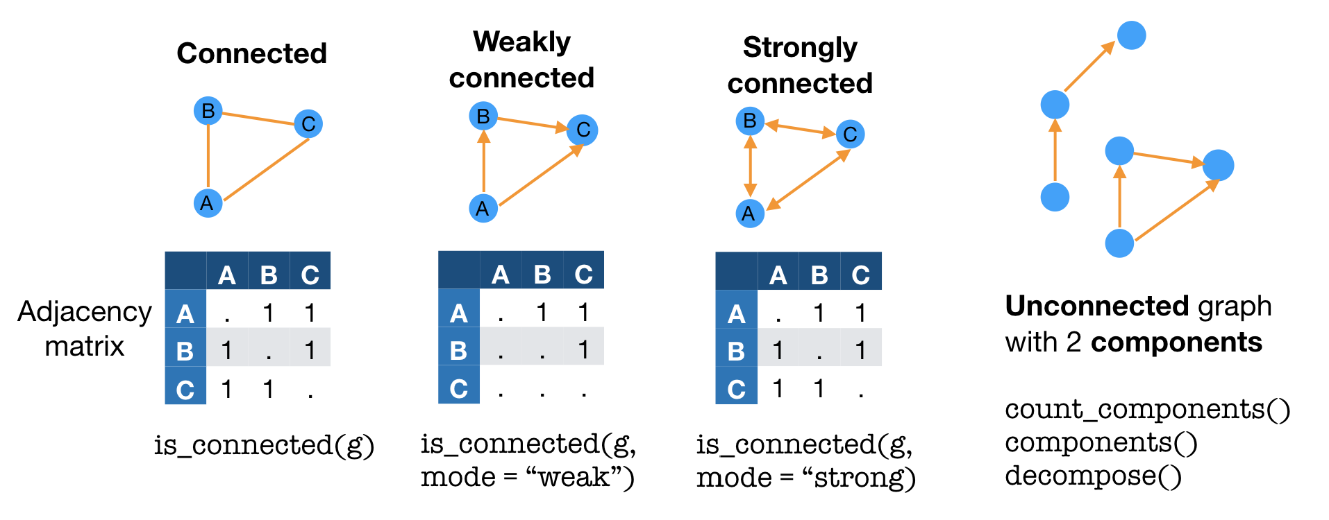
When all vertices of a graph are joined to each other via edges, a graph is considered to be connected. Directed graphs can be weakly connected when vertices are connected in one direction or strongly connected when vertices are connected bidirectionally. Graphs where vertices are not all joined are unconnected, with components that are connected.

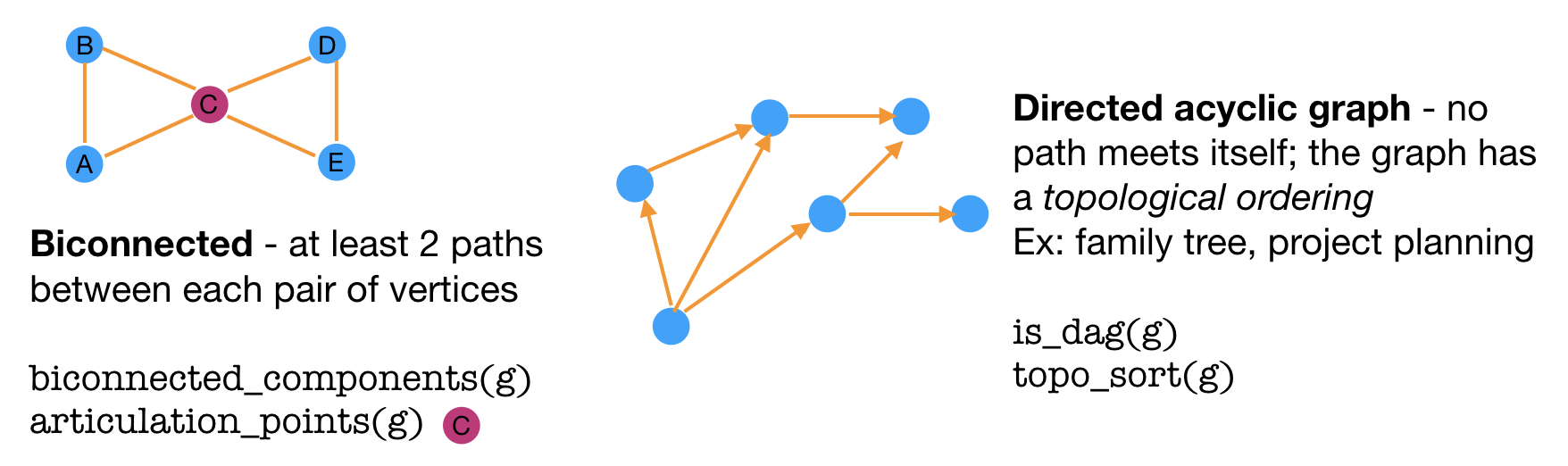
Some types of graphs come with special names. Biconnected graphs include at least 2 paths between each pair of vertices. A directed acyclic graph (DAG) is a graph without (“a-”) cyclic paths. That is, no matter what vertex you start on, any path will lead to one of the ending vertices without any repeat vertices.

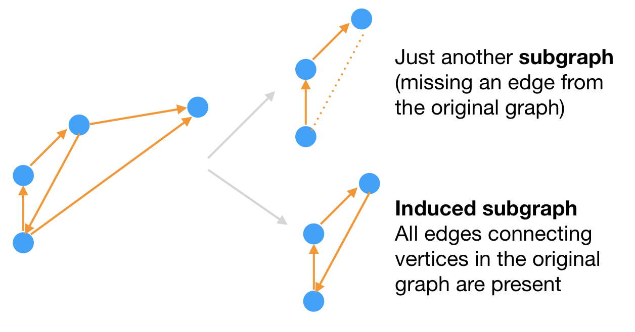
Sometimes, you may be interested in just a portion of the graph, or subgraph. A graph that contains all the vertices and all the edges from the original graph is an induced subgraph.

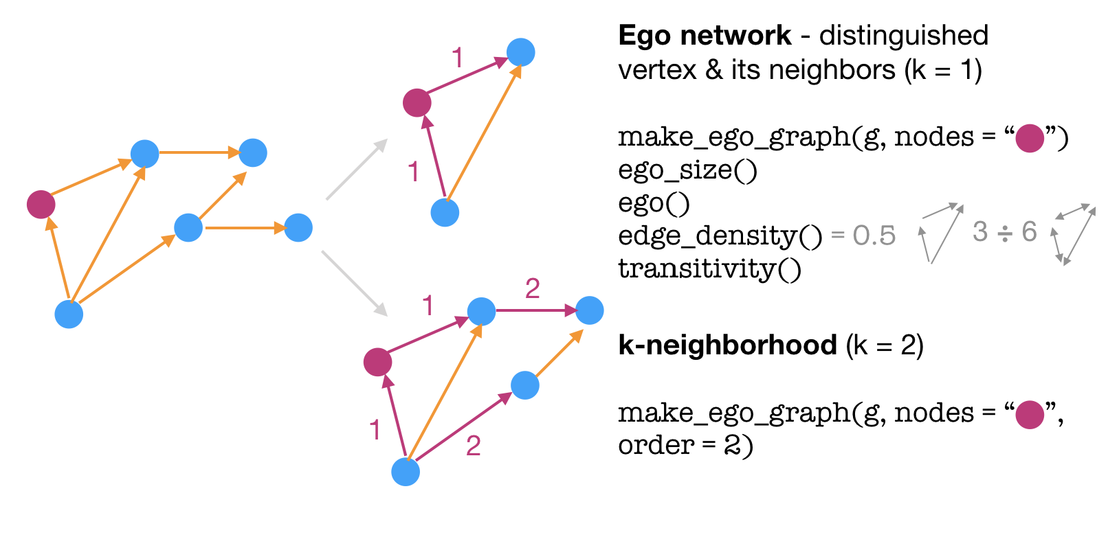
Another way to zoom in on a large graph is via an ego network, where you focus on a specific vertex and its closest neighbors.

That’s all folks!

There’s plenty more detail within the pdf book, but the rest will need to wait until another time!