The nitty-gritty of the Label Propagation Algorithm

library(tidyverse)

library(igraph) 
# many graph packages in R rely on igraph for computation
# lots of great functionality, sometimes confusing bc it's object-oriented 
# (it goes against my functional programming instincts)

# these packages marry graph data & tidyverse syntax
library(tidygraph)
library(ggraph)

head(highschool)

##   from to year
## 1    1 14 1957
## 2    1 15 1957
## 3    1 21 1957
## 4    1 54 1957
## 5    1 55 1957
## 6    2 21 1957

hs <- filter(highschool, year == 1957)

The endpoint

If I were to use label propagation normally, I’d use the following (fairly short) piece of code:

# igraph
g <- graph_from_data_frame(hs, directed = FALSE)
cluster_lpa <- cluster_label_prop(g)
cluster_lpa

## IGRAPH clustering label propagation, groups: 10, mod: 0.68
## + groups:
##   $`1`
##    [1] "1"  "2"  "3"  "6"  "9"  "12" "13" "14" "15" "20" "21" "22" "24" "29"
##   [15] "38" "51"
##   
##   $`2`
##   [1] "4"  "5"  "16" "18" "19"
##   
##   $`3`
##   [1] "7"  "8"  "17"
##   
##   + ... omitted several groups/vertices

plot(cluster_lpa, g)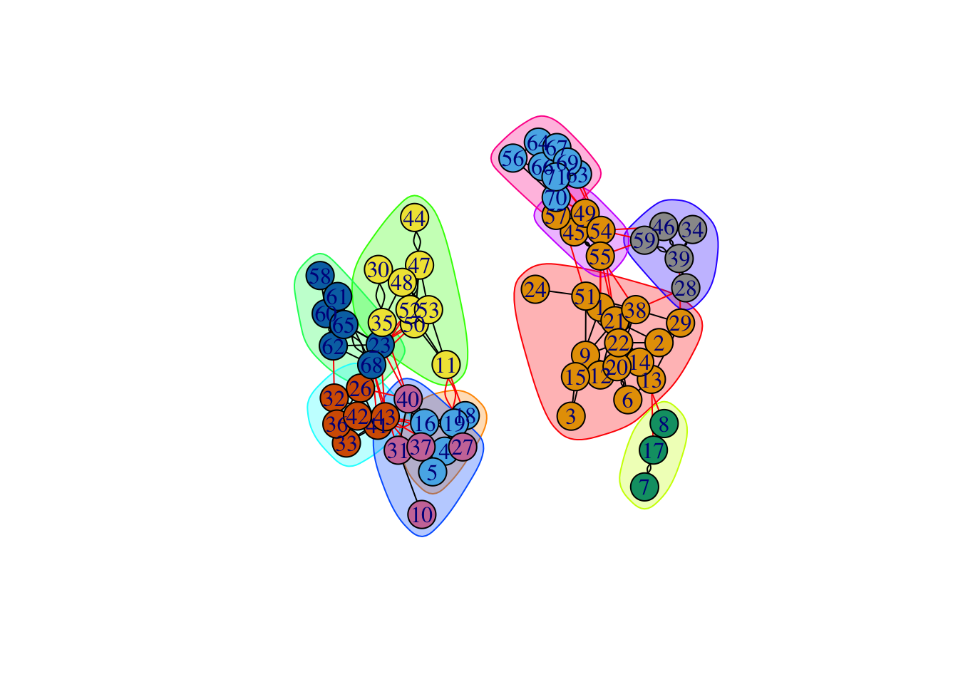

The “tidy” syntax is a bit more verbose, but if you already know ggplot/dplyr, it’s easy to know where to jump in to start tweaking.

# tidygraph / ggraph
g_tidy <- as_tbl_graph(hs) 

cluster_tidy_lpa <- g_tidy %>% 
    activate(nodes) %>% 
    mutate(group = group_label_prop()) 

ggraph(cluster_tidy_lpa) +
    geom_edge_link(color = "grey70") + #default is black
    geom_node_point(aes(color = as.factor(group)), size = 10) + #default is fairly small
    geom_node_text(aes(label = name)) +
    theme_void() +
    guides(color = FALSE, fill = FALSE)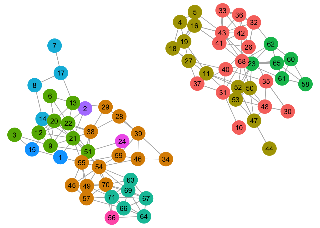 

For the rest of the plots, I’ll use the same layout and tweaked ggraph settings to make it easier to visually compare the results.

# this special layout object includes coordinates for each node
starting_layout <- create_layout(cluster_tidy_lpa, 
                                 layout = 'igraph', algorithm = 'kk')

create_ggraph <- function(graph_layout, node_color, label) {
    ggplot(graph_layout) +
        geom_edge_link(color = "grey70") +
        geom_node_point(aes(color = {{node_color}}), size = 10) +
        geom_node_text(aes(label = name)) +
        theme_void() +
        guides(color = FALSE) +
        scale_color_manual(values = scales::hue_pal()(15))
}

# once we have our group results, graph them all using the same layout
graph_cluster <- function(group_results, starting_layout) {
    layout_w_groups <- starting_layout %>%  
        left_join(rename(group_results, new = group), by = "name") %>% 
        mutate(name = fct_relevel(name, "22", "66", "36", "50", "45"),
               # use a few vertices to "anchor" the colors of certain groups
               name_int = as.integer(name)) %>% 
        mutate(new = fct_reorder(new, name_int, .fun = min))
    
    n_groups <- n_distinct(layout_w_groups$new)
    create_ggraph(layout_w_groups, node_color = new, label = name) +
        ggtitle(paste(n_groups, "clusters"))
}

The algorithm

Here, I’m aiming for the spirit of label propagation. For the specific details, go chase down some papers. These are my steps:

1. Starting state. The label propagation algorithm usually starts with a small set of labelled nodes. In our case, we’ll start without providing labels. Instead, each node will begin in a group of its own.
   
2. For each node, look at the groups of its neighbors. The most common group in the neighborhood (node + neighbors) becomes the node’s new group. In the case of a tie, sample randomly from the tied groups. This should result in a new group for each node. Normally nodes are randomly ordered and replaced as you go (“asynchronous”) – in my version, I’ll determine the new groups for all nodes and then replace them all at once (“synchronous”).
   
3. Compare new and old groups. If they are not the same, repeat step 2. The new group now becomes the “old”, or starting group, for step 2.

One important thing to note is that there’s an element of randomness at play, which means that results will differ per run. I didn’t bother to set any seeds here, but if you care about reproducibility, it’s probably a good idea.

Implementation

I’ll start with a bit of pseudo-code describing the steps above. We’ll rely on the graph data structure to store all our edge/node information, as well as tell us who the neighbors are.

edges 
nodes
graph <- to_graph(nodes, edges)

# every node starts in its own group
starting_groups <- nodes %>% mutate(group = 1:length(nodes)) 
groups_are_same <- FALSE

while(!groups_are_same) {
    # the map would have to be replaced with a for-loop in the async version
    new_groups <- map(nodes, ~determine_new_group(.x, starting_groups, graph))
    groups_are_same <- new_groups == starting_groups
    starting_groups <- new_groups
}

new_groups

The pseudocode doesn’t work yet, but it provides a structure to build off of. Now we just need to flesh out the pieces. We’ll start with some real data. In an effort to keep the code readable, I’m using variable names that are also igraph function names. Not ideal but going forward with it.

edges <- hs
graph <- as_tbl_graph(hs, directed = FALSE) #infers nodes from the edges
nodes <- graph %>% activate(nodes) %>% as_tibble() #extract dataframe of nodes

For the algorithm code, I’ve only had to make a few small changes to make it almost work. I’ve wrapped it in a run_lpa() function so we can easily run it multiple times. All we’re missing now is a determine_new_group() function that will return a data frame with new group.

run_lpa <- function(nodes, graph) {
    starting_groups <- nodes %>% mutate(group = row_number())
    groups_are_same <- FALSE
    
    while(!groups_are_same) {
        new_groups_vec <- map_chr(nodes$name, ~determine_new_group(.x, starting_groups, graph))
        groups_are_same <- identical(new_groups_vec, starting_groups$group)
        starting_groups <- starting_groups %>% 
            mutate(group = new_groups_vec)
    }
    
    starting_groups
}

Now let’s get into the the details of determining the new group for each node. I want to do the following:

1. Find all groups of its neighbors (+ its current group)
2. Choose the new group – if there is one most common group, it wins. If there are ties, then randomly sample from the tied groups.

Here is the coded version:

# step 1
get_neighborhood_groups <- function(node, starting_groups, graph) {
    neighbors <- make_ego_graph(graph, node = node)[[1]] %>% 
        V() %>% names()
    
    starting_groups %>% 
        filter(name %in% neighbors) %>% 
        pull(group)
}

# step 2
choose_group <- function(group_options) {
    all_counts <- table(group_options)
    max_counts <- all_counts[all_counts == max(all_counts)]
    if(length(max_counts) == 1) return(names(max_counts))
    names(sample(max_counts, size = 1))
}

# both steps together
determine_new_group <- function(node, starting_groups, graph) {
    neighbor_groups <- get_neighborhood_groups(node, starting_groups, graph)
    choose_group(neighbor_groups)
}

We’re pretty much done. Now to test it out:

lpa_output <- map(1:10, ~run_lpa(nodes, graph))
lpa_graphs <- map(lpa_output, graph_cluster, starting_layout = starting_layout) 

Graph comparison

How does my version compare to the igraph implementation? For convenience, we’ll use the tidygraph wrappers for the clustering functions. I’ll use the normalized mutual information metric (“nmi”) to igraph::compare() my 10 runs to the igraph LPA results I’ll also compare the runs to the edge betweenness and Louvain clustering results to get a better sense of how close I am.

lpa_nodes <- graph %>% 
    mutate(lpa = group_label_prop(),
           eb = group_edge_betweenness(),
           louvain = group_louvain()) %>% 
    as_tibble()

compare_nmi <- partial(compare, method = "nmi")
# new version of the function with the `method = "nmi"` saved

map(lpa_output, 
    ~tibble(lpa = compare_nmi(.x$group, lpa_nodes$lpa),
            eb = compare_nmi(.x$group, lpa_nodes$eb),
            louvain = compare_nmi(.x$group, lpa_nodes$louvain))) %>% 
    bind_rows(.id = "run")

## # A tibble: 10 x 4
##    run     lpa    eb louvain
##    <chr> <dbl> <dbl>   <dbl>
##  1 1     0.852 0.802   0.815
##  2 2     0.844 0.834   0.772
##  3 3     0.872 0.881   0.795
##  4 4     0.930 0.869   0.864
##  5 5     0.877 0.848   0.784
##  6 6     0.832 0.839   0.732
##  7 7     0.816 0.764   0.744
##  8 8     0.898 0.910   0.792
##  9 9     0.885 0.879   0.767
## 10 10    0.850 0.781   0.822

The normalized mutual information metric ranges from 0 to 1, where 1 means the communities are identical. My implementation is definitely closest to the LPA algorithm.

What if we just run LPA 10 times and compare it to the results of the three clustering algorithms above?

lpa_runs <- map(1:10, 
                ~graph %>% 
                    mutate(group = group_label_prop()) %>% 
                    as_tibble())

map(lpa_runs, 
    ~tibble(lpa = compare_nmi(.x$group, lpa_nodes$lpa),
            eb = compare_nmi(.x$group, lpa_nodes$eb),
            louvain = compare_nmi(.x$group, lpa_nodes$louvain))) %>% 
    bind_rows(.id = "run")

## # A tibble: 10 x 4
##    run     lpa    eb louvain
##    <chr> <dbl> <dbl>   <dbl>
##  1 1     0.950 0.907   0.858
##  2 2     0.971 0.969   0.920
##  3 3     0.981 0.939   0.891
##  4 4     0.982 0.921   0.872
##  5 5     0.964 0.921   0.872
##  6 6     0.981 0.939   0.891
##  7 7     0.982 0.921   0.872
##  8 8     0.983 0.922   0.873
##  9 9     0.965 0.904   0.854
## 10 10    0.952 0.949   0.836

The scores jumped up a bit – it’s possible my choice to update nodes synchronously rather than asynchronously is the cause of this difference. In any case, the point of this exercise was to dig deeper into the algorithm, rather than match the implementation exactly. And I can confidently say that my goal has been accomplished!