Rats to reefs

Tidy

To avoid crazy parsing gymnastics, I copied & pasted the text of the articles into *.txt files, which I’ve now uploaded onto GitHub. They still needed some cleaning, but it was a start.

library(tidyverse)
library(tidytext)
library(wordcloud)
library(pluralize) #devtools::install_github("hrbrmstr/pluralize")

atlantic <- readLines("https://raw.githubusercontent.com/isteves/website/master/static/post/2018-07-12-rats-to-reefs_files/ratsreef-atlantic.txt")
bbc <- readLines("https://raw.githubusercontent.com/isteves/website/master/static/post/2018-07-12-rats-to-reefs_files/ratsreef-bbc.txt")
nature <- readLines("https://raw.githubusercontent.com/isteves/website/master/static/post/2018-07-12-rats-to-reefs_files/ratsreef-nature.txt")

I decided to begin with just the Atlantic article to catch any funny business before going too deep into the analysis.

tibble(text = atlantic) %>% 
    unnest_tokens(word, text) %>% 
    anti_join(stop_words, by = "word") %>% 
    count(word, sort = TRUE) 

## # A tibble: 287 x 2
##    word         n
##    <chr>    <int>
##  1 â           17
##  2 islands     17
##  3 rats        12
##  4 rat         11
##  5 reefs        9
##  6 island       7
##  7 nitrogen     7
##  8 coral        6
##  9 free         6
## 10 found        5
## # ... with 277 more rows

Thanks to tidytext & tokenizers wizardry, the text is broken up into words with a few lines of code (borrowed from chapter 1 of the amazing Text Mining with R by Julia Silge and David Robinson!). We can see right away that:

• we’ve got strange garbles such as â
• I’ve got words that differ only in plurality (rats versus rat)
• and if I scroll through the list some more, some of the “words” are actually numbers

With an extra lines of stringr and the fantastic pluralize package, I can fix these problems.

tibble(text = atlantic) %>% 
    mutate(text = str_replace_all(text, "[^a-zA-Z]", " ")) %>% 
    # replace anything NOT (^) in the alphabet with a space
    
    unnest_tokens(word, text) %>% 
    anti_join(stop_words, by = "word") %>% 
    mutate(word = singularize(word)) %>% #from the pluralize package
    
    count(word, sort = TRUE) 

## # A tibble: 244 x 2
##    word           n
##    <chr>      <int>
##  1 island        26
##  2 rat           24
##  3 reef          11
##  4 coral         10
##  5 graham         8
##  6 seabird        8
##  7 nitrogen       7
##  8 free           6
##  9 difference     5
## 10 found          5
## # ... with 234 more rows

It looks pretty good! Now let’s functionalize it and repeat it for the other two articles. While I’m at it, let me also add in a column for the source.

clean_text <- function(text, source) {
    tibble(source = source,
           text = text) %>% 
        mutate(text = str_replace_all(text, "[^a-zA-Z]", " ")) %>%
        unnest_tokens(word, text) %>%
        anti_join(stop_words, by = "word") %>%
        mutate(word = singularize(word)) %>% 
        group_by(source) %>% # need this to keep the source column
        count(word, sort = TRUE)
}

With map2, I can then apply the function to my three texts and bind them together.

all_words <- map2(list(atlantic, bbc, nature),
                  list("atlantic", "bbc", "nature"),
                  clean_text) %>% 
    bind_rows()

Visualize

Now for some #dataviz. I love looking at word clouds, so let’s take a look at a couple here. The word size in these visualizations represents the relative abundance (count) in the text. Since the original Nature article is much longer than the two news articles, let’s look at it separately.

all_words %>% 
    filter(source == "nature") %>% 
    with(wordcloud(word, n, max.words = 100))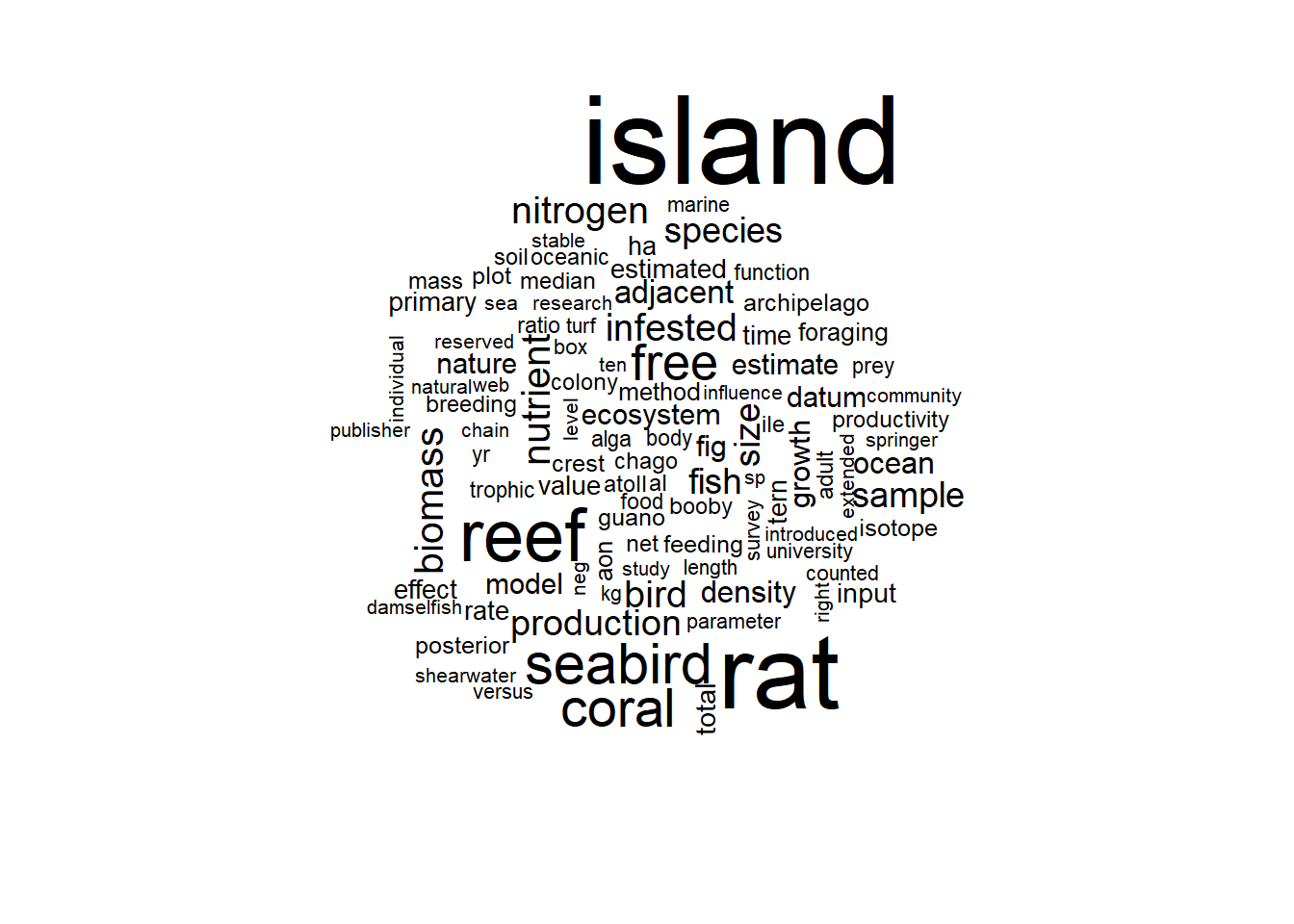

Island, rat, and reef clearly dominate. We see that some weird-looking words appear in the cloud. Some of those appear to be units (kg, yr) and others belong to longer phrases (al) but don’t usually stand alone. For the purpose of the blogpost, it’s good enough. (Though don’t do this for your thesis!)

If we compare all three, we find that the BBC put the strongest emphasis on the impact on coral reefs.

all_words %>% 
    reshape2::acast(word ~ source, value.var = "n", fill = 0) %>% 
    comparison.cloud(colors = c("#0072B2", "#D55E00",  "#009E73"),
                     max.words = 100)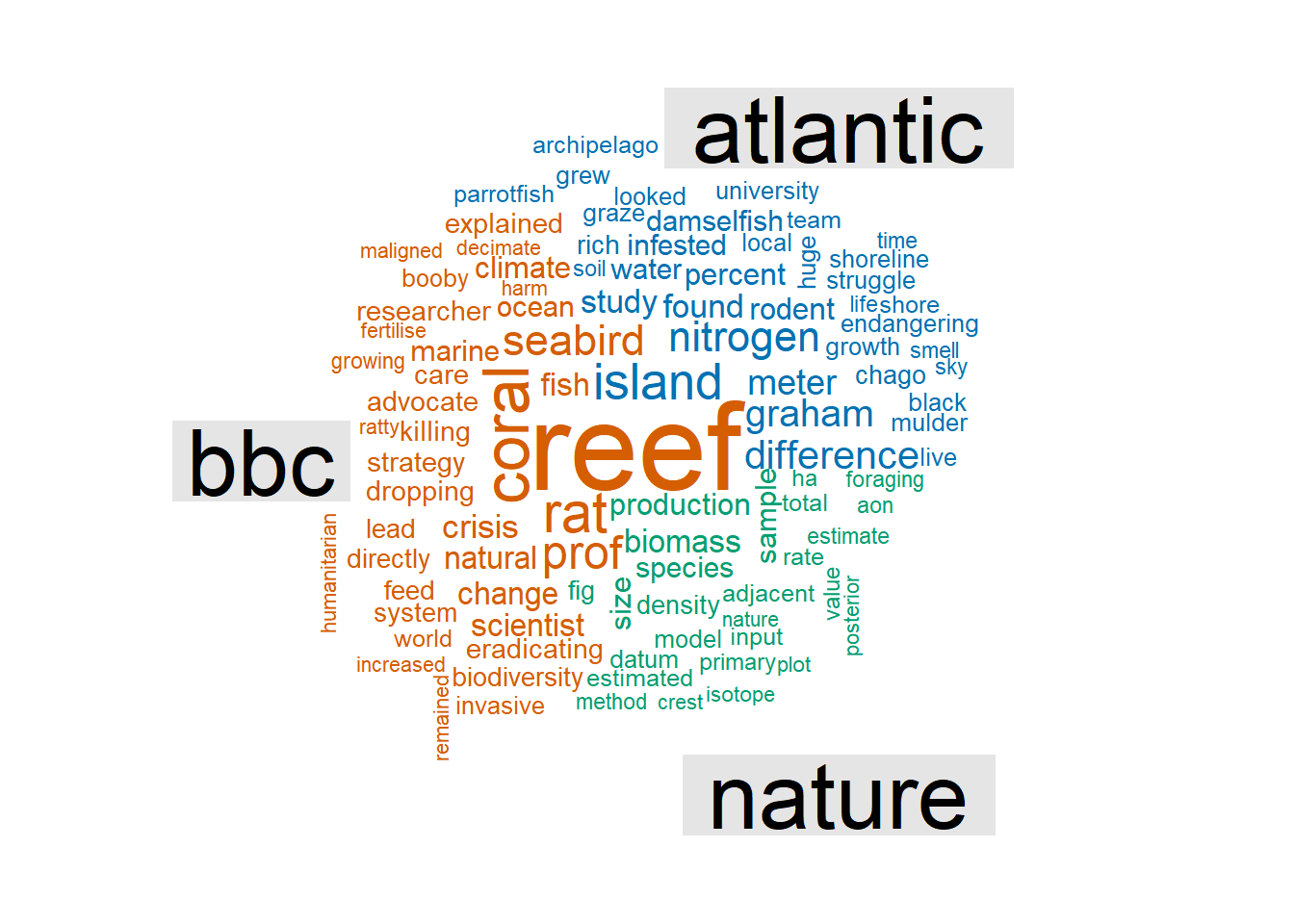

We can look at this more directly using bar graphs. Here, I take the 10 most common words from each article, and see how they compare across sources. In this case, the x-axis scale is auto-adjusted so that we can better compare the relative counts.

top_words <- all_words %>% group_by(source) %>% top_n(10)

all_words %>% 
    filter(word %in% top_words$word) %>% 
    ggplot(aes(fct_reorder(word, n), n)) +
    geom_col() +
    xlab(NULL) +
    coord_flip() +
    facet_wrap(~ source, scales = "free_x")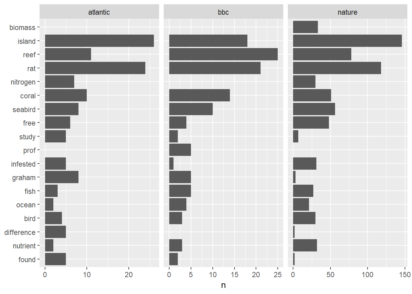

As expected, “island,” “rat,” and “reef” are commonly used in the three articles with “coral” and “seabird” following closely behind.

The original article stresses biomass, whereas the news articles focus on the scientists themselves (“Prof Graham”, in the case of the BBC). Interestingly, the BBC article makes no mention of nitrogen and instead uses a variety of more colloquial words, such as “nutrients,” “fertilizer,” and “droppings.”

all_words %>% 
    mutate(single_word = ifelse(n == 1, TRUE, FALSE)) %>% 
    group_by(source, single_word) %>% 
    summarize(count_word = n())

## # A tibble: 6 x 3
## # Groups:   source [?]
##   source   single_word count_word
##   <chr>    <lgl>            <int>
## 1 atlantic FALSE               50
## 2 atlantic TRUE               194
## 3 bbc      FALSE               40
## 4 bbc      TRUE               146
## 5 nature   FALSE              563
## 6 nature   TRUE               812

Conclusion

As I reread the two news articles again, I find that the difference in word use are highlighted in the authors’ disparate strategies in telling the story.

Victoria Gill from the BBC is succinct and to the point. Each paragraph contains no more than two sentences, and she lays out the story in two sections: “How do rats harm coral reefs?” and “Why does this matter?” The latter section is almost entirely about the importance of coral reefs generally, which explains the heavy use of reef that we saw above.

In contrast, Ed Yong uses longer-form prose to highlight the historical and academic landscape of the study. He writes about humans inadvertently carrying rats to the islands in the late 18th and early 19th centuries, and describes the complex and abundant relationships among members of this ecosystem. Like Victoria Gill, Ed Yong ends on a conservation note: eradicating rats from islands is “low-hanging fruit” as far as management actions are concerned.

Graham et al.’s study pulled together a lot of smaller studies into a cohesive and compelling story, but the best part of is definitely Aaron MacNeil’s GitHub link to the analyses and plots! Way to champion reproducible research!