In my recent exploration of window functions, I realized didn’t really know the differences between rank functions. The dplyr documentation lists out six functions, of which I pretty much only use one (row_number()):
row_number()ntile()min_rank()dense_rank()percent_rank()cume_dist()
Though the documentation description is relatively clear, it was still hard to grasp exactly how they differed. I found it easier to do the comparison visually.

Trivia score ranks
Given a toy dataset of trivia scores from two teams, let’s see how the scores rank using the functions above.
library(tidyverse)
theme_set(theme_minimal())

set.seed(20200417) #so I get the same teams each time
trivia_scores <- tibble(team = sample(c("cheetah", "ibex"), 10, replace = TRUE),
                        score = c(3, 6, 6, 18, 39, 40, 40, 40, 42, 99))

window_rank_example <- trivia_scores %>%
    mutate(ntile3 = ntile(score, 3),
           min_rank = min_rank(score),
           dense_rank = dense_rank(score),
           percent_rank = percent_rank(score) %>% round(3),
cume_dist = cume_dist(score)) | team | score | ntile3 | min_rank | dense_rank | percent_rank | cume_dist |
|---|---|---|---|---|---|---|
| ibex | 3 | 1 | 1 | 1 | 0 | 0.1 |
| ibex | 6 | 1 | 2 | 2 | 0.111 | 0.3 |
| ibex | 6 | 1 | 2 | 2 | 0.111 | 0.3 |
| cheetah | 18 | 1 | 4 | 3 | 0.333 | 0.4 |
| ibex | 39 | 2 | 5 | 4 | 0.444 | 0.5 |
| cheetah | 40 | 2 | 6 | 5 | 0.556 | 0.8 |
| ibex | 40 | 2 | 6 | 5 | 0.556 | 0.8 |
| ibex | 40 | 3 | 6 | 5 | 0.556 | 0.8 |
| cheetah | 42 | 3 | 9 | 6 | 0.889 | 0.9 |
| cheetah | 99 | 3 | 10 | 7 | 1 | 1 |
From the patterns above we see that:
- the distances between scores don’t matter (39 to 40 is treated the same way as 42 to 99)
- all except for
ntile()clump the three 40’s together into one team min_rank()reaches 10 (the total number of scores) whereasdense_rank()reaches 7 (the total number of distinct scores)percent_rank()is similar tomin_rank()except that (a) it ranges from 0 to 1 and (b) each step is 0.111 instead of 1- each step of
cume_dist()is 1 / # scores (1/10 = 0.1 in this case) and is similar tomin_rank()except that all ties get the maximum score
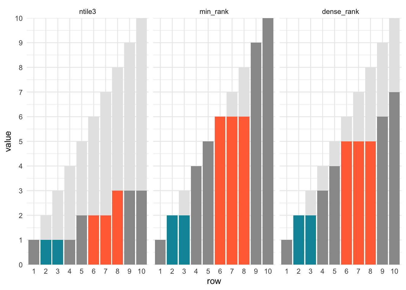
To dig into it even more, here’s another way of visualizing the ranks. Since ranks are only dependent on the order of values and not the value itself (except with repeats), I’ve used row number for the x-axis and added it as a light gray background as well.
We see that with the exception of ntile, all ranking functions group repeated numbers together (I colored the two 6’s in teal and the three 40’s in orange).

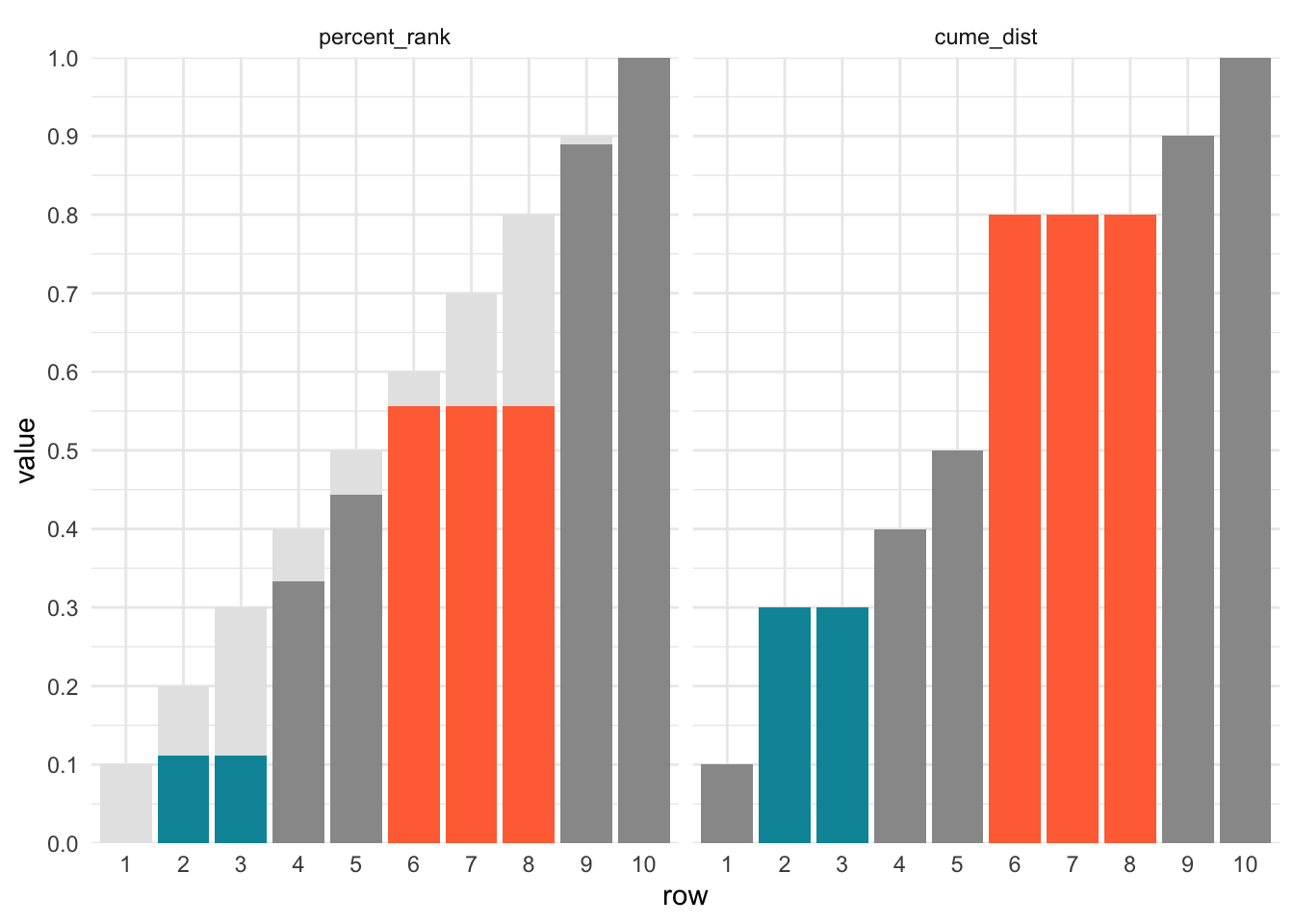
Since percent_rank() and cume_dist() reach a maximum of 1, I decided to plot them separately. The light gray background indicates equal increments of 0.1 across all 10 values.

Ranking per group
Splitting by team requires just one extra line (and one more to make the resulting table look nicer):
window_rank_example_teams <- trivia_scores %>%
    group_by(team) %>% # only change needed!
    arrange(team, score) %>% # not required but easier to digest visually
    mutate(ntile3 = ntile(score, 3),
           min_rank = min_rank(score),
           dense_rank = dense_rank(score),
           percent_rank = percent_rank(score) %>% round(3),
cume_dist = cume_dist(score)) | team | score | ntile3 | min_rank | dense_rank | percent_rank | cume_dist |
|---|---|---|---|---|---|---|
| cheetah | 18 | 1 | 1 | 1 | 0 | 0.25 |
| cheetah | 40 | 1 | 2 | 2 | 0.333 | 0.5 |
| cheetah | 42 | 2 | 3 | 3 | 0.667 | 0.75 |
| cheetah | 99 | 3 | 4 | 4 | 1 | 1 |
| ibex | 3 | 1 | 1 | 1 | 0 | 0.166666666666667 |
| ibex | 6 | 1 | 2 | 2 | 0.2 | 0.5 |
| ibex | 6 | 2 | 2 | 2 | 0.2 | 0.5 |
| ibex | 39 | 2 | 4 | 3 | 0.6 | 0.666666666666667 |
| ibex | 40 | 3 | 5 | 4 | 0.8 | 1 |
| ibex | 40 | 3 | 5 | 4 | 0.8 | 1 |
Now, instead of overall ranks, the scores for each team are ranked separately.
Reversing ranks
Perhaps you think it’s weird that the lowest trivia scores get the highest rank (1). To reverse the ranking order, we can use either desc() or just add a -.
window_rank_example_reversed <- trivia_scores %>%
    mutate(ntile3 = ntile(-score, 3),
           min_rank = min_rank(-score),
           dense_rank = dense_rank(-score),
           percent_rank = percent_rank(-score) %>% round(3),
cume_dist = cume_dist(-score)) | team | score | ntile3 | min_rank | dense_rank | percent_rank | cume_dist |
|---|---|---|---|---|---|---|
| ibex | 3 | 3 | 10 | 7 | 1 | 1 |
| ibex | 6 | 3 | 8 | 6 | 0.778 | 0.9 |
| ibex | 6 | 3 | 8 | 6 | 0.778 | 0.9 |
| cheetah | 18 | 2 | 7 | 5 | 0.667 | 0.7 |
| ibex | 39 | 2 | 6 | 4 | 0.556 | 0.6 |
| cheetah | 40 | 1 | 3 | 3 | 0.222 | 0.5 |
| ibex | 40 | 1 | 3 | 3 | 0.222 | 0.5 |
| ibex | 40 | 2 | 3 | 3 | 0.222 | 0.5 |
| cheetah | 42 | 1 | 2 | 2 | 0.111 | 0.2 |
| cheetah | 99 | 1 | 1 | 1 | 0 | 0.1 |
Conclusion
And that’s all there is to it! Hope the visual aids help to reinforce the differences in the options.